The Amazon Web Services network has 69 locations worldwide in 22 regions: USA, Europe, Asia, Africa and Australia. In each zone there are up to 8 data centers – Data Processing Centers. Each data center has thousands or hundreds of thousands of servers. The network is built in such a way that all unlikely outage scenarios are taken into account. For example, all regions are isolated from each other, and access zones are spaced several kilometers apart. Even if you cut the cable, the system will switch to backup channels, and information loss will amount to units of data packets. About what other principles the network is built and how it is built, will tell you below.

Our technical advice will help you live and grow in the AWS cloud.

In this part, we will focus on network scaling – one of the most complex systems in AWS. Evolution from a flat network to Virtual Private Cloud and its device, internal Blackfoot and HyperPlane services, the problem of a noisy neighbor, and in the end – the scale of the network, backbone and physical cables.

Network scaling

AWS Cloud launched in 2006. Its network was quite primitive – with a flat structure. The range of private addresses was common to all tenants of the cloud. When you start a new virtual machine, you accidentally received an available IP address from this range.

This approach was easy to implement, but fundamentally limited the use of the cloud. In particular, it was quite difficult to develop hybrid solutions that combined private networks on the ground and in AWS. The most common problem was the intersection of ranges of IP addresses.

Virtual private cloud

The cloud was in demand. It was time to think about the scalability and the possibility of its use by tens of millions of tenants. Flat network has become a major obstacle. Therefore, we thought about how to isolate users from each other at the network level so that they can independently select IP ranges.

What comes to mind first when you think about network isolation? Of course VLAN and VRF – Virtual Routing and Forwarding.

Unfortunately, this did not work. VLAN ID is only 12 bits, which gives us only 4096 isolated segments. Even in the largest switches, you can use a maximum of 1-2 thousand VRF. The combined use of VRF and VLAN gives us just a few million subnets. This is definitely not enough for tens of millions of tenants, each of which should be able to use several subnets.

We also simply cannot afford to buy the required number of large boxes, for example, from Cisco or Juniper. There are two reasons: it is furiously expensive, and we do not want to become dependent on their development and patch policies.

In 2009, we announced VPC – Virtual Private Cloud. The name has taken root and now many cloud providers also use it.

VPC is a Software Defined Network (SDN) virtual network. We decided not to invent special protocols at the L2 and L3 levels. The network runs on standard Ethernet and IP. For transmission over a network, virtual machine traffic is encapsulated in a wrapper of our own protocol. It indicates the ID that belongs to the Tenant VPC.

That sounds easy. However, it is necessary to solve several serious technical problems. For example, where and how to store mapping data for virtual MAC / IP addresses, VPC IDs, and the corresponding physical MAC / IP. On an AWS scale, this is a huge table that should work with minimal latency. The mapping service, which is  a thin layer throughout the network, is responsible for this.

In machines of new generations, encapsulation is performed by Nitro cards at the hardware level. In older instances, encapsulation and decapsulation are software.

Let’s see how this works in general terms. Let’s start with level L2. Suppose we have a virtual machine with IP 10.0.0.2 on a physical server 192.168.0.3. It sends data to a 10.0.0.3 virtual machine that lives on 192.168.1.4. An ARP request is generated, which falls on the Nitro network card. For simplicity, we believe that both virtual machines live in the same “blue” VPC.

• The card replaces the source address with its own and sends the ARP frame to the mapping service.
• The mapping service returns the information that is needed for transmission over the L2 physical network.
• The nitro card in the ARP response replaces the MAC in the physical network with the address in the VPC.
• When transferring data, we wrap the logical MAC and IP in a VPC wrapper. All this is transmitted over the physical network using the appropriate IP Nitro source and destination cards.
• The physical machine the package is intended to perform checks. This is to prevent the possibility of change. The machine sends a special request to the mapping service and asks: “From the physical machine 192.168.0.3 I received a packet that is designed for 10.0.0.3 in the blue VPC. Is it legitimate?”
• The mapping service checks its resource allocation table and allows or denies the passage of the packet. In all new instances, additional validation is stitched in Nitro cards. It is impossible to get around even theoretically. Therefore, spoofing to resources in another VPC will not work.
• Then the data is sent to the virtual machine for which it is intended.

The mapping service also works as a logical router for transferring data between virtual machines on different subnets. Everything is conceptually simple there, I will not analyze it in detail.

It turns out that during the transmission of each packet, the servers access the mapping service. How to deal with inevitable delays? Caching, of course.

You do not need to cache the entire huge table. Virtual machines from a relatively small number of VPCs live on a physical server. Information needs to be cached only about these VPCs. Transferring data to other VPCs in the “default” configuration is still not legitimate. If functionality such as VPC-peering is used, information about the corresponding VPCs is additionally loaded into the cache.

With the transfer of data to the VPC figured out.

Blackfoot

What to do in cases when traffic needs to be transmitted outside, for example, on the Internet or through a VPN to the ground? This is where Blackfoot, the AWS internal service, helps us out. It is designed by South African team. Therefore, the service is named after the penguin who lives in South Africa.

Blackfoot decapsulates the traffic and does what it needs with it. Internet data is sent as is.

The data is decapsulated and wrapped again in an IPsec wrapper when using a VPN.

When using Direct Connect, traffic is tagged and transmitted to the corresponding VLAN.

HyperPlane

This is an internal flow control service. Many network services require data flow status monitoring. For example, when using NAT, flow control should ensure that each “IP: destination port” pair has a unique outgoing port. In the case of the NLB balancer – Network Load Balancer, the data stream should always be directed to the same target virtual machine. Security Groups is a stateful firewall. It monitors incoming traffic and implicitly opens ports for the outgoing packet stream.

In the AWS cloud, transmission latency requirements are extremely high. Therefore, HyperPlane is critical to the health of the entire network.

Hyperplane is built on EC2 virtual machines. There is no magic here, only cunning. The trick is that they are virtual machines with large RAM. Transactions are transactional and performed exclusively in memory. This allows for delays of only tens of microseconds. Working with a disk would destroy all the performance.

Hyperplane is a distributed system of a huge number of such EC2 machines. Each virtual machine has a bandwidth of 5 GB / s. Across the entire regional network, this gives terabits of bandwidth and allows you to process millions of connections per second.

HyperPlane only works with threads. VPC packet encapsulation is completely transparent to him. The potential vulnerability in this internal service will still not allow breaking through VPC isolation. For safety, the levels below are responsible.

Noisy neighbor

There is still the problem of a noisy neighbor. Suppose we have 8 nodes. These nodes carry out flows of all users of a cloud. Everything should be evenly distributed across all nodes. The nodes are very powerful and difficult to overload.

We build our architecture even from improbable scenarios.

We can imagine a situation in which one or more users will generate too much load. All HyperPlane nodes are involved in processing this load, and other users can potentially feel some kind of performance degradation. This destroys the concept of a cloud in which tenants have no way to influence each other.

How to solve the problem of a noisy neighbor? The first thing that comes to mind is sharding. Our 8 nodes are logically divided into 4 shards with 2 nodes in each. Now, a noisy neighbor will be hindered by only a quarter of all users, but much more.

Let’s do it differently. Each user is allocated only 3 nodes.

The trick is to assign nodes to different users randomly. In the picture below, the blue user intersects the nodes with one of the other two users – green and orange.

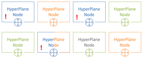
With 8 nodes and 3 users, the probability of a noisy neighbor crossing with one of the users is 54%. With this probability that the blue user will affect other tenants. Moreover, only a part of its load. In our example, this effect will be at least somehow noticeable not to everyone, but only a third of all users. This is already a good result.

Let’s bring the situation closer to the real one – take 100 nodes and 5 users on 5 nodes. In this case, none of the nodes intersects with a probability of 77%.

In a real situation with a huge number of HyperPlane nodes and users, the potential impact of a noisy neighbor on other users is minimal. This method is called shuffle sharding. It minimizes the negative effect of node failure.

Many services are built on the basis of HyperPlane: Network Load Balancer, NAT Gateway, Amazon EFS, AWS PrivateLink, AWS Transit Gateway.

Network scale

Now let’s talk about the scale of the network itself. For October 2019, AWS offers its services in 22 regions, and 9 more are planned.

•     Each region contains several Availability Zones. There are 69 of them in the world.
•     Each AZ consists of Data Processing Centers. There are no more than 8 of them.
•     The data center houses a huge number of servers, some of which up to 300,000.

Now all this averaged, multiplied and get an impressive figure that displays the scale of the Amazon cloud.

Between the access zones and the data center, many optical channels are laid. In one of our largest regions, only 388 channels have been laid for the communication of AZ between themselves and communication centers with other regions (Transit Centers). In total, this gives 5000 Tbit.

Backbone AWS is built specifically for the cloud and optimized to work with it. We build it on 100 GB / s channels. We fully control them, with the exception of regions in China. Traffic is not shared with the loads of other companies.

Of course, we are not the only cloud provider with a private backbone network. More and more large companies are going this way. This is confirmed by independent researchers, for example, from Telegeography.

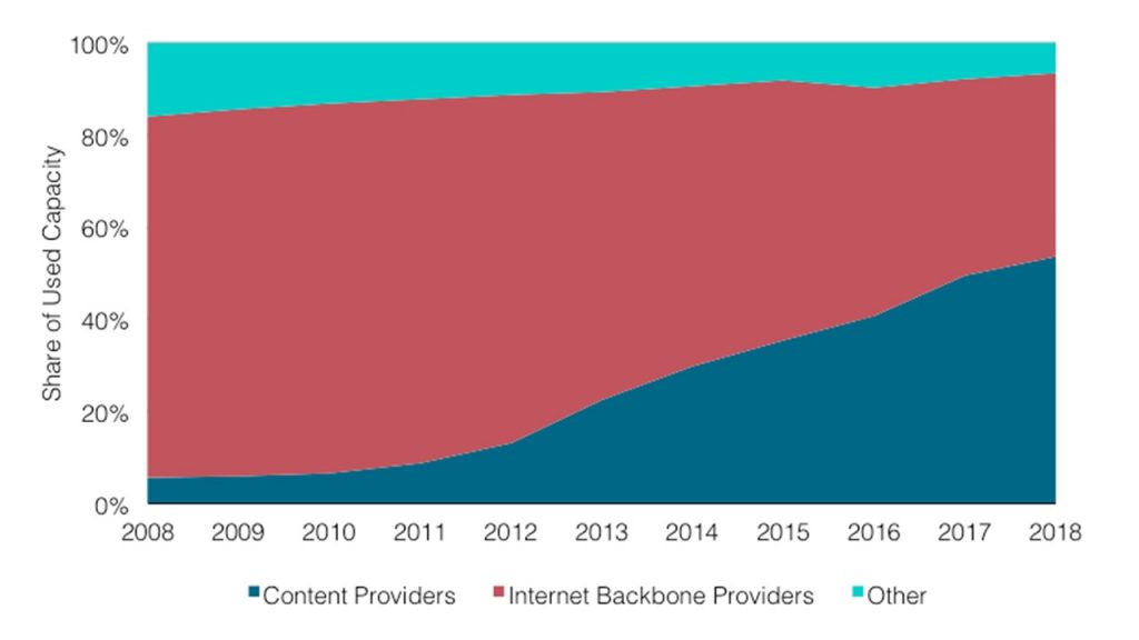The graph shows that the share of content providers and cloud providers is growing. Because of this, the proportion of Internet traffic from backbone providers is constantly decreasing.

I will explain why this happens. Previously, most web services were available and consumed directly from the Internet. Now more and more servers are located in the cloud and are available through the CDN – Content Distribution Network. To access the resource, the user goes through the Internet only to the nearest CDN PoP – Point of Presence. Most often it is somewhere nearby. Then he leaves the public Internet and flies through the Atlantic via a private backbone, for example, and gets directly to the resource.

Physical channels

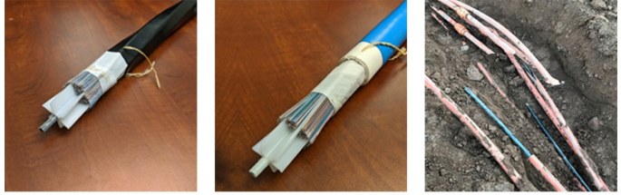
Scientists have not yet figured out how to increase the speed of light in the Universe, but have made great advances in the methods of transmitting it through optical fiber. We are currently using 6912 fiber cables. This helps to significantly optimize the cost of their installation.

In some regions we have to use special cables. For example, in the Sydney region, we use cables with a special coating against termites.

No one is safe from troubles and sometimes our channels are damaged. The photo on the right shows optical cables in one of the American regions that were torn by builders. As a result of the accident, only 13 data packets were lost, which is surprising. Once again – only 13! The system literally instantly switched to backup channels – the scale works.

We had a look over some Amazon cloud services and technologies. I hope that you have at least some idea of ​​the scale of the tasks that our engineers have to solve. Personally, I am very interested in this.